
Today has been a day to reflect on the way things actually work and the perverse outcomes that sometimes obtain when we do what seems logical…meaning, of course, that unintended consequences are everywhere.
—–
Over the past 20 years or so, perhaps more, environmental advocacy groups (Environmental Defense, Sierra Club, etc.) have trained their guns on industrial agriculture, especially industrial ANIMAL agriculture, arguing that the larger our “animal factories” (their term, not mine!) become, the greater risk they pose to the environment. The logical conclusion they reach is that the livestock and poultry industries need to be regulated more and more heavily.
It should be obvious to anyone who thinks about it for even a moment that an increase in regulatory intensity nearly always results in significantly increased costs of regulatory compliance. Those may include the professional labor costs of defending against newly enabled litigation, or the capital and operating costs of additional pollution-control technologies, or the administrative costs of generating more piles of paperwork to be filed and copied and shipped, or all three and many more.
It’s also obvious that increased labor, capital, operating, and administrative costs are all nothing more or less than increased costs of producing a marketable product. The “animal factory” now costs more to run per unit of livestock produced than it did prior to the increased regulatory intensity. Profit margin shrinks.
Naturally, the producer wants to stay in business. It’s pretty well understood that if a business’ profit margin is shrinking, one way to reverse that is to get larger, to increase capacity. That is what we call “economies of scale,” and it is one of the main reasons (no doubt) that Tortilleria Lupita now occupies at least four facilities in Amarillo instead of just one. And McDonald’s. And Chick-Fil-A. Why did we go from the old, brown Wal-Marts to the big, blue, Super Wal-Marts? Economies of scale are at least one of the main reasons. We spread fixed costs over more units of production, and the decline in profit margin can be reversed.
—–
Wait, though! Wasn’t the big, bad “animal factory” the problem we set out to solve in the first place? And yet: what we’ve just done is describe an interesting perversity that lurks in “the way things actually work.” We set out to turn the screws on large “animal factories,” hoping – vainly, as it turns out – to incentivize a return to mom-and-pop agriculture, happy cows on green pasture, free-range chickens, and all the rest. But what we actually DID was incentivize further concentration of animal units in these “animal factories.”
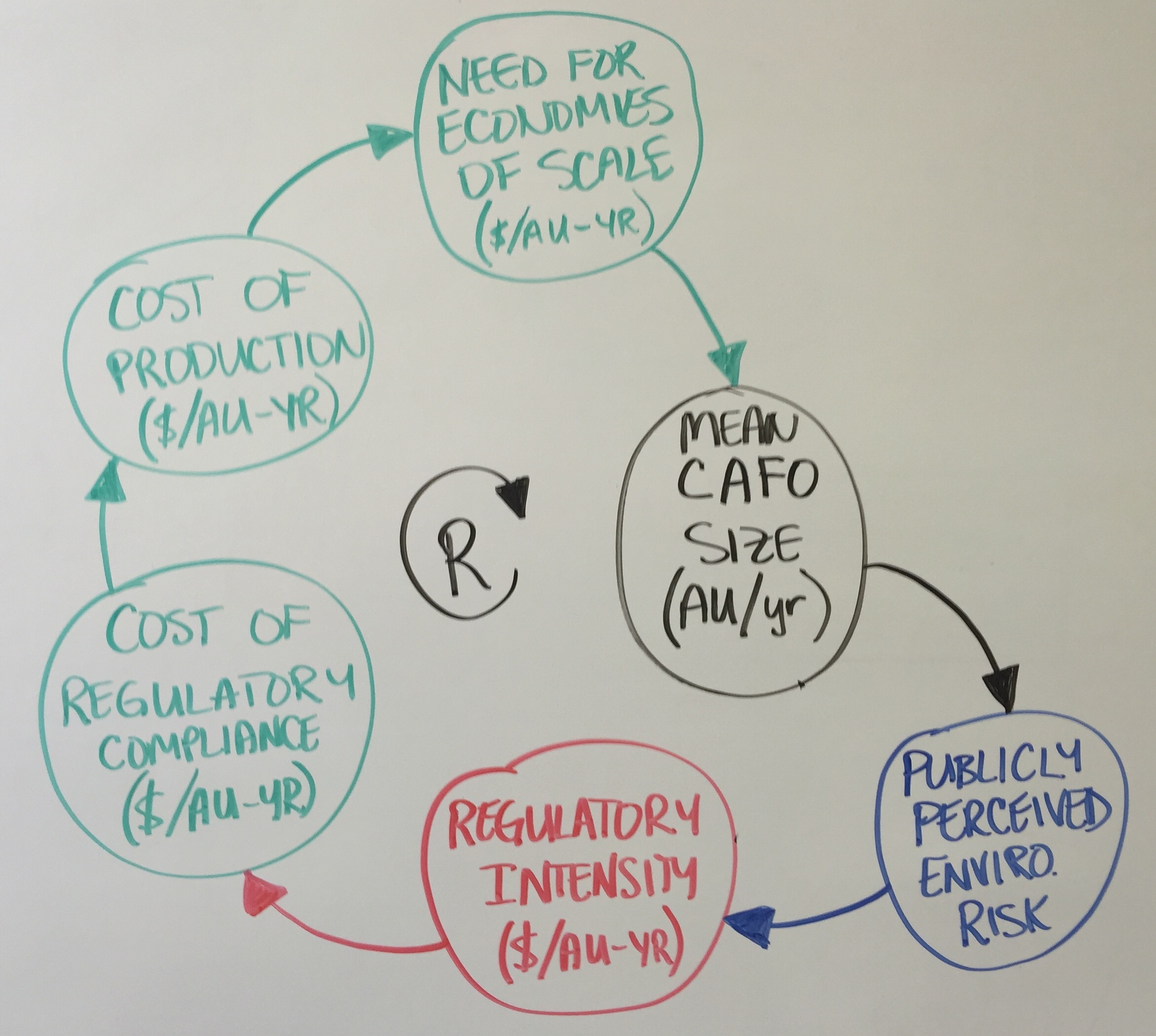
A reinforcing feedback loop helps to drive the intensification of the livestock and poultry industries.
—–
So what’s the answer? First, let’s get a couple of things straight. We can afford a juicy steak (or, for you vegans, a fresh, juicy strawberry in the dead of winter) precisely because we have industrialized agriculture. Have you tried growing your own strawberries around here in January? And you may have noticed that if you want a Kobe filet, you’d better be independently wealthy. For the rest of us, that corn-fed NY strip from a Kansas or Texas feedyard may not be an everyday meal, but you probably don’t have to take out a mortgage to enjoy one every once in a while. Prime Kobe beeves may be flown across the Pacific on 747s, but a choice, English-cross steer only has to be rolled a few miles on a semi. Be thankful.
Second, these are not the only dynamics at play. I’ve just isolated this particular dynamic to show how it works. In truth, lots of other things are going on at the same time this reinforcing loop is executing.
Third, we can probably conclude that, all other things being equal, a large-scale producer is more able to afford (i. e., absorb the costs of without going bankrupt) a government-mandated increase in environmental protection than the small-scale producer. That’s the way it is. The selection pressures are mostly in favor of the larger, more robust, industrial model…
—–
Mostly. But that’s a discussion for another day.