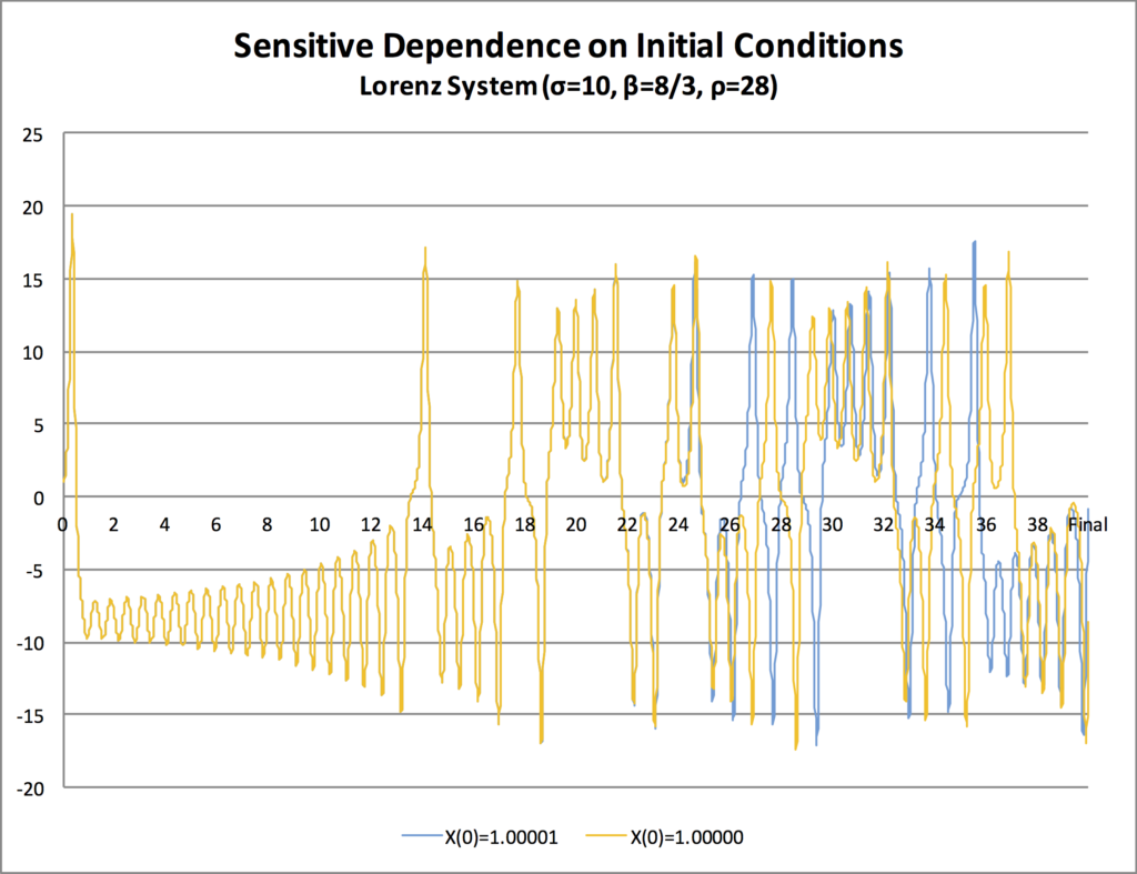
With the relentless media-academia assault on so-called “climate-change deniers” – a defamatory, misleading term if ever there was one – I am always and ever reflecting on why I continue to cast my lot with the skeptics. And I nearly always end up back here, pondering the graph below.
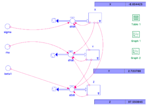
I’ve been preparing to teach an ultra-short course on Stella [TM] modeling at a conference in North Carolina next month. (Stella is a simulation platform for complex systems, a simple way to simulate a system’s evolution over time.) In preparation for that workshop, I decided to put together a Stella model of the “Lorenz system,” a highly simplified version of a system of equations that Dr. Edward Lorenz derived to describe atmospheric dynamics back in the early 1960s. With a bunch of simplifying assumptions, the system reduces to an ensemble of three short equations that are easily solved by a computer.

Two simulations of the same Lorenz system, with only a 0.001% difference between the initial values of X.
The computers they had then were extremely crude, of course, and quite slow by modern standards. A simulation my Mac can handle in 20 seconds used to take many days. Lorenz would run his simulations in stages; he’d run a simulation for a long work day, print out the appropriate data, and start a new simulation the next day, starting at the point he had stopped the simulation on the previous day. Perfectly logical, right? Except he noticed something odd.
The computer he was using actually retained numbers at pretty high precision. Let’s say the internal storage held the number 3.208945992. When he printed his data at the end of each day, his output format only extended to four or five decimals, rounding the number accordingly: 3.20895, let’s say. So the next day, when starting the simulation, he would enter 3.20895, which the computer interpreted as 3.20895000, a difference from the number the computer had actually held at the end of the previous day’s run. The difference between the two, in this case, is 0.000004008, which is an error of about 0.00001%. No big deal, right?
When he noticed he was inserting these tiny, tiny errors into the simulation, he was interested in how much of an effect they had. So he ran one simulation continuously for a period of days, never stopping the computer. He then repeated the simulation from exactly the same starting point, but he stopped and started the simulation daily as I described earlier. And what he found was, some might argue, the birth of modern “chaos theory.”
The two simulations tracked along very, very closely for several days. After a few days, some small divergences appeared, but they didn’t seem to amount to much. But then…the two simulations went completely in different directions.
I’ve done a similar thing with my Stella model of the Lorenz system this morning. The system tracks the evolution of three variables, X, Y, and Z. The system requires that the initial values of all three variables be specified. In my first simulation, I set X=1.00000, Y=1.00000, and Z=1.00000 at the outset. In my second simulation, I kept the exact same values for Y and Z, but I changed X to 1.00001. Then I ran each simulation exactly the same way.
Just as Lorenz found, the first half of the simulation yielded no detectable difference between the two scenarios. In fact, you can’t even see the blue line because it’s directly behind the yellow line. But look what happens after that! The two graphs diverge a little, then a bit more, and then they go in completely different directions!
Now you’re asking: so what?
Keep in mind that much climate science depends on numerical models much more complicated, with many more variables, than the Lorenz system. Climate models involve averaging some kinds of data over very large areas, say, 1 km x 1 km squares of land or sea area. Even if we had 100 weather stations in that square, there is no way to be sure that the average value of the variable X computed from the measurements of X at each weather station would represent the “true” average value of X over the grid. In fact, the very notion of a “true” average value of X is itself kinda funny; each of the weather stations’ sensors is slightly different, each generates its own errors (by definition), and we can’t measure X at each point in the grid, especially with only 100 weather stations. So an error of .00001% is not hard to imagine, is it?
But look what happened when Lorenz made such an error in specifying his initial conditions for a particular daily run!
Later that year, he published a research paper in which he concluded,
Two states differing by imperceptible amounts may eventually evolve into two considerably different states … If, then, there is any error whatever in observing the present state—and in any real system such errors seem inevitable—an acceptable prediction of an instantaneous state in the distant future may well be impossible….In view of the inevitable inaccuracy and incompleteness of weather observations, precise very-long-range forecasting would seem to be nonexistent.
In other words, there’s a limit to how accurate our atmospheric models can be. We can be fairly accurate in the short run, but long-range forecasting is doomed.
BTW, don’t bother with the “weather is not climate” thing. I know that. But both involve atmospheric dynamics, and if we can’t simulate weather with great confidence, why would we expect to simulate climate with any better confidence?
Does that mean we shouldn’t do it? Of course not. But we ought to be humble about the accuracy of any long-range projections and forecasts of complex, dynamic systems like the earth’s atmosphere.

